Parametrically controlled terrain generation

The intent was to produce a single mountain while ensuring as much control as possible over the resulting terrain through algorithmic parameters. I ended up with this algorithm that allows you to specify desired coordinate of the mountain, height of the mountain peak and spread of the base region.

This algorithm is inspired by my previous work, the RMP algorithm and the famous Fault line algorithm by R. Krten. The algorithm takes three parameters as input. The number of fault lines l, probing depth r and number of iterations to perform n. The relationship between these parameters and physical properties of the mountain is a little complex. Height of the peak is directly proportional to n, spread of the mountain base is function of l,r and steepness of the mountain is inversly proportional to r.

These images bellow are result of tweaking with n parameter, notice the difference in height.



With a little modification introduced, the same procedure can produce craters and other unusual artifacts as well, as can be seen in these images.



The work was published in GRAPHITE 2007 bearing title Parametrically Controlled Terrain Generation.

Artificial Terrain Generation : RMP

These are results of Repeated Magnification and Probing algorithm for generating artificial terrain. The algorithm itself is pretty basic, and the results are pretty much basic height maps. But these can be used as base maps for erosion algorithms to produce nice realistic results.





The work was published as,

Repeated Magnification : a New Approach to Generating Artificial Mountain like Terrain
4th International Conference on Computer Graphics and Interactive Techniques in Australasia and Southeast Asia ( GRAPHITE 2006 ) Kuala Lumpur, Malaysia

Updates on Sea Turtle Species ID

Had considerable progress in this month on my ongoing research work, the sea turtle species identification project. Can detect two sea turtle species now among the seven species of sea turtles. Here are test results for two pictures of sea turtle carcasses found washed up on coast of Bangladesh. the one on top is Lepidochelys olivacea(LO) a.k.a Olive Ridley and the one bellow is Chelonia mydas(CM) a.k.a Green turtle. The white line around the subject and the name of species in black letters inside the black box at top-left corner are output produced by my program.

Click the links for more on species ID of Olive Ridley and Green turtles.

Image courtesy : M.A. Hannan

Smoothing image historgram in MATLAB

%load rgb image
src = 'C:\rainbow.jpg';
rgbI = imread(src);
grayI = rgb2gray(rgbI);

%get image histogram
[counts bins]=imhist(grayI);

%fit histogram into polynomial to get smooth curve
fit = polyfit(bins,counts,10);
fit_samples = polyval(fit,bins);

%show histogram
plot(bins,counts,'.g',bins,fit_samples,'-b');


Image histogram in MATLAB


%load rgb image
src = 'C:\rainbow.jpg';
rgbI = imread(src);
grayI = rgb2gray(rgbI);

%get image histogram
[counts bins]=imhist(grayI);

%show histogram
bar(bins,counts);


RGB to Lab color transformation in MATLAB


%load rgb image
src = 'C:\rainbow.jpg';
rgbI = imread(src);

%convert to lab
labTransformation = makecform('srgb2lab');
labI = applycform(rgbI,labTransformation);

%seperate l,a,b
l = labI(:,:,1);
a = labI(:,:,2);
b = labI(:,:,3);

figure, imshow(l) , title('l');
figure, imshow(a) , title('a');
figure, imshow(b) , title('b');


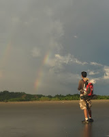
The input image


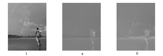
and the output







image courtesy : Ashraful Alam

Directory listing in MATLAB

For listing files in a directory

dirfullname = 'C:\Documents and Settings\';
fileFolder = fullfile(dirfullname);
dirOutput = dir(fullfile(fileFolder));
fileNames = {dirOutput.name}'


To filter files, use the second argument of fullfile function.

dirOutput = dir(fullfile(fileFolder,'*.jpg'));