Video of Information visualization workshop at SUST

This is a video clip of me teaching a class at the Information visualization workshop in SUST at 28th February 2010. This clip only shows Halo among the many information visualization techniques I discussed about.



Hope this will be helpful to my students. Apologies for not so good videography.

Lab color model is preferred for computer vision

For working with computer vision and image processing, I prefer using Lab to other popular color models like RGB and CMYK. Unlike the RGB and CMYK color models, Lab color is designed to approximate human vision. It aspires to perceptual uniformity. Perceptually uniform means that a change of the same amount in a color value should produce a change of about the same visual importance. The L compoent in Lab closely matches human perception of lightness while a and b components represent stimulation along the color opponent dimensions of red-green and blue-yellow respectively.



The Lab color space is a color-opponent space. The color opponent theory states that the human visual system interprets color information by processing signals from cones and rods in an antagonistic manner. The three types of cones have some overlap in the wavelengths of light to which they respond, so it is more efficient for the visual system to record differences between the responses of cones, rather than each type of cone's individual response. The opponent color theory suggests that there are three opponent channels: red versus green (a component in Lab), blue versus yellow (b component in Lab), and black versus white (L component in Lab). Responses to one color of an opponent channel are antagonistic to those to the other color.

Gasteracantha Arcuata : Bizarre looking spider in Lawachhora

Found this bizarre looking spider in Lawachhora forest. It was a late autumn morning on 29th November, 2010. A little research on the internet after coming back home reveals that this spider belongs to the genus Gasteracantha. The common name is Spiny-backed orb-weavers or Spiny orb-weavers because of their spiny abdomen and ability to weave vertical orb webs.



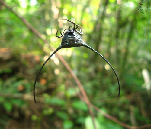
The observed specimen belongs to the species Gasteracantha arcuata. It has two long curved spines on its back and black/dark gray color all over. According to the sources on the internet[*], this species is found in Malaysia, Indonesia, Thailand, India and China. Sightings of this species in Bangladesh is probably not well documented. From my last expedition to Lawachhora forest however, it is evident that this species is abundant in that area.

I'm planning an expedition for collecting more information on this species and documenting its behavior. Hopefully I'll meet these critters in Lawachhora again at the end of December, 2010.

Here are some more photos of this species found on the internet.

References

http://www.malaeng.com/blog/?p=10612
http://godofinsects.com/museum/display.php?sid=121

Planner graph on Kemp Ridley and Olive Ridley turtles' carapace

Kemp's Ridley or Lepidochelys kempii is the smallest of all sea turtle species. Reaching maturity at 2–3 feet (61–91 cm) long and averaging only 45 kilogram. It's carapace contains five vertebral scutes running down the midline, while five pairs of costal scutes border them. The resulting planar graph due to this scalation is 3-regular 28 vertices and 42 edges. Exactly same as as that of Loggerhead or Caretta Caretta.



Olive Ridley or Lepidochelys olivacea is also one of the smallest turtle species. its heart-shaped carapace is characterized by four pairs of pore-bearing inframarginal scutes on the bridge, two pairs of prefrontals, and up to nine lateral scutes per side. Scalation can be asymmetrical i.e. 6 lateral scutes on one side and 8 on the other.

Planner graph on Loggerhead Turtle's carapace

The Loggerhead sea turtle or Caretta Caretta is the world's largest hard-shelled turtle. It's carapace contains five vertebral scutes running down the midline, while five pairs of costal scutes border them. The resulting planar graph due to this scalation is 3-regular 28 vertices and 42 edges.

Planner graph on Green Turtle's carapace

In graph theory, a planar graph is a graph that can be embedded in the plane, i.e., it can be drawn on the plane in such a way that its edges intersect only at their endpoints.

A graph is said to k-regular if all the vertices of the graph has dgree k.



The Green sea turtle or Chelonia mydas has a dorsoventrally flattened body. Its carapace is composed of five central scutes flanked by four pairs of lateral scutes. The resulting planner graph is 3-regular with 24 vertices and 36 edges.

Histogram smoothing with erosion

The idea of using erosion for smoothing histogram is actually borrowed from the realm of artificial terrain generation where it is a common practice. Recent experiments shows this is a better approach then using polynomial fit. Histogram is a one dimensional height map, after all. The result (smoothed histogram) closely follows the actual data points most of the time and structural property like rises and falls are well preserved.



The procedure is pretty straight forward, replace each entry in the vector containing the histogram with mean of that entry along with n entries backwards n entries forward. Boundary case arises when the index of the current entry is bellow n or beyond length_of_vector-n, I chose to keep those entries unchanged.

    result = arr ;

    for i=n+1:length(arr)-n
        sum=0;
        for j=i-n:i+n
            sum = sum + arr(j) ;
        end
        result(i) = sum/(2*n+1);
    end

Sea turtle carapace pattern as criterion for automatic species ID

The pattern seen on the carapace of sea turtles is one of the criterion used for identifying species, why not try to use this for automatic species ID as well ? The advantages of using this approach for automatic ID would be

1. Works for photos taken in wide range of environments and lighting condition varying from the animal's natural habitat (under water) to decaying carcass of stranded animals found on beaches
2. Only the carapace needs to be observed; other body parts, which decay sooner than the carapace in a dead animal, don't need to be observed
   
3. Can work for both color and bw photographs
4. Possibility of successful detection from broken or incomplete carapace if the key parts of the carapace is found

However, the challenges associated with this approach are also great. The challenges are encountered in two different phases, each of them are explained bellow.

• Feature Extraction
  The sought after feature here is the pattern on the carapace. To understand the challenges in extracting this feature, we should understand its origin first. What we are referring to as pattern in common English as 'Pattern' is actually the network of ridge lines between scutes on the turtles carapace. This is true for all the species of Cheloniida family. For Dermochelys coriacea or leatherback turtle, the only species of Dermochelyidae family, the pattern is originated by the seven ridge lines on its back. Experimentation with several photograph taken in varying environment reveals that the ridge lines are best visible, hence extractable, in case of underwater photos.
  
  
  
  The above image shows the result of gradient magnitude, a standard edge detection algorithm, applied on a photograph followed by edge thinning on the resulting gradient magnitude image. But this does not yield good extractable features from photographs of stranded animals found on beaches, specially the decaying ones. Worse, due to presence of debris or other objects inside the frame, wrong part of the image is extracted instead of the carapace by the gradient magnitude finding operation.
  
  




• Graph reconstruction
  The next challenge encountered is reconstruction of the pattern extracted from the photograph. Ideally, this would be the complete network of ridge lines. But the resulting image after feature extraction does not always have a complete network traced in most of the real life situations. So the graph reconstruction procedure should be robust enough to reconstruct a graph from incomplete or broken edges and at the same time be able to identify and discard edges that are not from the ridge lines on the turtles back.
  

Graph on sea turtle carapace

Sea turtles belong to the superfamily Chelonioidea and inhabit all of the world's oceans except the Arctic. There are seven species of sea turtles.

Family Cheloniida

Chelonia mydas or green turtle
Eretmochelys imbricata or hawksbill turtle
Natator depressus or flatback Turtle
Caretta caretta or Loggerhead Sea Turtle
Lepidochelys kempii or Kemp's Ridley turtle
Lepidochelys olivacea or Olive Ridley turtle

Family Dermochelyidae

Dermochelys coriacea or leatherback turtle



The above Image shows how to identify species of a sea turtle based on its carapace or the back. Anyone with idea of Graph theory would immediately recognize the graphs drawn on the carapace of different turtle species. I believe this is a good criterion for automated species identification from sea turtle photographs.

Parametrically controlled terrain generation

The intent was to produce a single mountain while ensuring as much control as possible over the resulting terrain through algorithmic parameters. I ended up with this algorithm that allows you to specify desired coordinate of the mountain, height of the mountain peak and spread of the base region.

This algorithm is inspired by my previous work, the RMP algorithm and the famous Fault line algorithm by R. Krten. The algorithm takes three parameters as input. The number of fault lines l, probing depth r and number of iterations to perform n. The relationship between these parameters and physical properties of the mountain is a little complex. Height of the peak is directly proportional to n, spread of the mountain base is function of l,r and steepness of the mountain is inversly proportional to r.

These images bellow are result of tweaking with n parameter, notice the difference in height.



With a little modification introduced, the same procedure can produce craters and other unusual artifacts as well, as can be seen in these images.



The work was published in GRAPHITE 2007 bearing title Parametrically Controlled Terrain Generation.

Artificial Terrain Generation : RMP

These are results of Repeated Magnification and Probing algorithm for generating artificial terrain. The algorithm itself is pretty basic, and the results are pretty much basic height maps. But these can be used as base maps for erosion algorithms to produce nice realistic results.





The work was published as,

Repeated Magnification : a New Approach to Generating Artificial Mountain like Terrain
4th International Conference on Computer Graphics and Interactive Techniques in Australasia and Southeast Asia ( GRAPHITE 2006 ) Kuala Lumpur, Malaysia

Updates on Sea Turtle Species ID

Had considerable progress in this month on my ongoing research work, the sea turtle species identification project. Can detect two sea turtle species now among the seven species of sea turtles. Here are test results for two pictures of sea turtle carcasses found washed up on coast of Bangladesh. the one on top is Lepidochelys olivacea(LO) a.k.a Olive Ridley and the one bellow is Chelonia mydas(CM) a.k.a Green turtle. The white line around the subject and the name of species in black letters inside the black box at top-left corner are output produced by my program.

Click the links for more on species ID of Olive Ridley and Green turtles.

Image courtesy : M.A. Hannan

Smoothing image historgram in MATLAB

%load rgb image
src = 'C:\rainbow.jpg';
rgbI = imread(src);
grayI = rgb2gray(rgbI);

%get image histogram
[counts bins]=imhist(grayI);

%fit histogram into polynomial to get smooth curve
fit = polyfit(bins,counts,10);
fit_samples = polyval(fit,bins);

%show histogram
plot(bins,counts,'.g',bins,fit_samples,'-b');


Image histogram in MATLAB


%load rgb image
src = 'C:\rainbow.jpg';
rgbI = imread(src);
grayI = rgb2gray(rgbI);

%get image histogram
[counts bins]=imhist(grayI);

%show histogram
bar(bins,counts);


RGB to Lab color transformation in MATLAB


%load rgb image
src = 'C:\rainbow.jpg';
rgbI = imread(src);

%convert to lab
labTransformation = makecform('srgb2lab');
labI = applycform(rgbI,labTransformation);

%seperate l,a,b
l = labI(:,:,1);
a = labI(:,:,2);
b = labI(:,:,3);

figure, imshow(l) , title('l');
figure, imshow(a) , title('a');
figure, imshow(b) , title('b');


The input image


and the output







image courtesy : Ashraful Alam

Directory listing in MATLAB

For listing files in a directory

dirfullname = 'C:\Documents and Settings\';
fileFolder = fullfile(dirfullname);
dirOutput = dir(fullfile(fileFolder));
fileNames = {dirOutput.name}'


To filter files, use the second argument of fullfile function.

dirOutput = dir(fullfile(fileFolder,'*.jpg'));